Parallelizing Haskell Raytracer
This is just a translation of my article from 2023. Stylistic choices of the original are mostly retained. It will not be substantially expanded upon, but I do feel this article could benefit from better methodology. More on that later. You can read original in russian here: https://luxurious-yearde9.notion.site/Parallel-Haskell-raytracer-63132332960f488aaa04b7cc01e13f8e.
Introduction
So we made a raytracer in haskell using Raytracing In One Weekend as our guide. As you may know, haskell’s biggest feature is mathematically correct functions. Meaning the result of the evaluation can be determined solely from the arugments. So no more global or hidden state. This computing models lends itself great to parrallel execution. However there were a few unexpected pitfalls that I want to share.
While measuring performance benefit of parallelizing I also became interested in how fast it can go. Hence a second part about optimisations.
All of the code is available at https://github.com/TheBlek/haskell-raytracer
Baseline measurements
For all measurements I’m going to use three configurations:
Small: 11.33s (Avg 3)
Medium: 94.5s (Avg 3)
Big: 408.93s (Just 1)
Everything later will be measured one-shot.
Threads go brrr
Having downloaded package parallel, I replaced following line:
write_file "output.ppm" (evalState colors (mkStdGen 0))
with
write_file "output.ppm" (evalState colors (mkStdGen 0) `using` parList rseq)
Just calculating an array of colors for each pixel in parallel. And…
12 seconds for small configuration…
And I could see only one thread in htop.
That’s because mutlithreading needs to be turned on at compile time:
ghc-options:
    -threaded
    -rtsopts
    -with-rtsopts=-N -- Can pass number of threads to limit (-N4)
Now we are ready to take off!
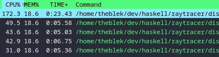
Looking good!
Wait, what?…
24 seconds on the small test?… From baseline of 11.3?!
Something’s wrong here.
This might happen because of resource contension between threads. And we actually have a resource that we “share” - random number generator. We can’t generate random numbers for one pixel until we have done so for previous pixel. Otherwise numbers will be the same for each pixel and won’t be random. And empirically that leads to artifacts in the image. So what do we when we actually want to share?
Looking at this code now in 2025, I’m not sure anymore what caused such a massive slowdown. Maybe it’s because of spawning so many thread simutaneously? I mean, obviously, it wasn’t “sharing”. Remember - no direct sharing in haskell. However, fundamentally we needed to share pRNG. And that certainly is a limiter. I’m not even sure what the code written the first time parallelized…
Our case is pretty simple - we can create any number of pRNGs and use each of them sequentially:
let accumulated_color = [multi_color objs u v (floor samples_per_pixel)|
            v <-  reverse [0, 1/(image_height - 1)..1],
            u <-  [0, 1/(image_width - 1)..1]]

let len = image_height * image_width
let part_len = len / 4
let map_colors = mapM (fmap (adjust_gamma 2 . average samples_per_pixel))
let st_colors = map map_colors (chunksOf (floor part_len) accumulated_color)

let colors_parts = zipWith (\st i -> evalState st (mkStdGen i)) st_colors [0..]
let colors = concat (colors_parts `using` parList rseq)
write_file "output.ppm" colors
Running small test we get 13 seconds. That’s better, but still bad. What am I doing wrong?
Haskell is a lazy capybara
Turns out, problem was because of haskell does not evaluate anything immediately. It stores objects that describe the calculation that is evaluated on demand.
ghci> let x = 1 + 2 :: Int
ghci> :sprint x
x = _
ghci> seq x ()
()
ghci> :sprint x
x = 3
That also applies to constructors of types:
ghci> let x = 1 + 2 :: Int
ghci> let z = swap (x, x+1)
ghci> :sprint z
z = _
ghci> seq z ()
()
ghci> :sprint z
z = (_,_)
As you can notice, field values remain uncomputed. As it turns out, seq will not go deeper than one level. To compute field values, you need to demand them:
ghci> fst z
4
ghci> :sprint z
z = (4,3)
In this case, first field (x + 1) was dependent upon evaluation of x so haskell automatically calculated x. And second field happened to be x, hence its evaluated.
The function that we used to calculate list in parallel - parList - just uses seq on each of the list element in parallel. You can probably see the problem:
data Color = Cl {color::Vec3}
---
ghci> let color = blue
ghci> :sprint color
color = _
ghci> seq color ()
color = Cl _
---
[Cl _, Cl _, ...]
And actual colors were calculated when function writing the image needed them.
For solving this problem there is a class RNFData in the deepseq package. This class has a single function that has to make haskell evaluate a value completely. For parallelizing computation of colors we needed to specify the behaviour for our types:
instance NFData Color where
    rnf (Cl x) = rnf x

instance NFData Vec3 where
    rnf (Vc3 x y z) = seq x $ seq y $ seq z ()
Then replace one line:
let colors = concat (colors_parts `using` parList rdeepseq)
And finally a W:
Small: 8s (~1.41x)
Medium: 64s (~1.47x)
Big: 277s (~1.48x)
For a machine with two real cores, the result looks as expected. Seeing those numbers stired up my interest in optimisations.
Optimisations go brrr
Still threads
On the previous step we divided colors into 4 parts because my working machine had 4 threads, but is it optimal?
So I decided to check two other divisions: by rows and by columns. With typical screen ratio 16 by 9, that would make more columns than rows.
Note, from here on out I will specify speedup in parethesis relative to previous-best results.
Row split:
Small: 7.13s (1.12x)
Medium: 57.95s (1.10x)
Big: 260s (1.07x)
Column split:
Small: 7.12s (1.12x)
Medium: 62.8s (1.02x)
Big: 249s (1.11x)
As you can see, column and row splits give results within a margin of error. However its clear that its better to divide on more parts than just 4.
The easiest
Easiest optimisation are just compiler flags:
-funfolding-use-threshold=16
-optc-O3
-optc-ffast-math
-fspecialise-aggressively
-fexpose-all-unfoldings
"-with-rtsopts=-N -s -A64M"
This gives us:
Small: 6.61s (1.078x)
Medium: 55.9s (1.055x)
Big: 233.9s (1.069x)
Its not much, but its honest work. Especially not having done anything :)
Wizardry
In search of further optimisation opportunities I run the program under a profiler to see which functions are the heaviest or hottest. First two lines are not surprising unlike next three. Sure, we are doing a lot of Vec-number multiplications, but why are they not inlining?
Note: «* and *» are our operators to multiply 3d vector with a number
COST CENTRE         MODULE                    %time %alloc
sphere_intersection Hittable                  16.2   13.5
hit_dist            Hittable                  16.1   12.7
<<*                 Vec3                      6.1   11.3
length_sqr          Vec3                      6.0    5.1
*>>                 Vec3                      5.2    5.0
hit_nearest_sph     Hittable                  4.1    4.7
scatter             Material                  4.0    3.7
randomRS            MyRandom                  3.8    4.3
color_ray           Main                      3.7    3.5
hit_point           Hittable                  3.1    3.9
hit_dist            Hittable                  3.0    3.0
hit_normal          Hittable                  3.0    1.9
random_vec          MyRandom                  2.8    4.0
+                   Vec3                      2.7    2.3
atPoint             Ray                       2.5    3.3
multi_color         Main                      2.2    2.3
gen_ray             Main                      1.9    2.5
headMay             Safe                      1.2    0.0
hit_data            Hittable                  1.1    0.4
reflect             Material                  1.0    1.3
blend               Color                     0.9    1.7
<<\                 Vec3                      0.9    1.2
nextWord64          System.Random.SplitMix    0.8    3.6
absorb              Color                     0.6    1.2
Well, lets help the compiler aka do the work for it by inserting INLINE statements on all vector operations:
{-# INLINE (*>>) #-}
{-# INLINE (<<*) #-}
{-# INLINE (<<\) #-}
{-# INLINE dot #-}
{-# INLINE length_sqr #-}
Results:
Small: 4.93s (1.34x)
Medium: 40.68s (1.37x)
Big: 173.24s (1.35x)
Wow! This speedup is comparable with going mutltithreading! 5 lines gave ~35%! But wait, there is more. Resulting program can be profiled again:
COST CENTRE           MODULE                 %time %alloc

hit_dist              Hittable               20.5   15.4
sphere_intersection   Hittable               11.4   16.6
randomRS              MyRandom               5.5    5.2
hit_nearest_sph       Hittable               5.5    5.7
color_ray             Main                   5.1    4.1
hit_normal            Hittable               4.8    3.8
scatter               Material               4.7    3.7
hit_point             Hittable               4.4    5.5
hit_dist              Hittable               3.9    3.7
random_vec            MyRandom               3.8    4.9
gen_ray               Main                   3.2    3.1
atPoint               Ray                    3.1    4.0
norm                  Vec3                   3.1    6.0
multi_color           Main                   3.1    2.8
+                     Vec3                   2.4    1.6
headMay               Safe                   1.6    0.0
hit_data              Hittable               1.6    0.5
absorb                Color                  1.4    1.5
-                     Vec3                   1.2    0.9
reflect               Material               1.2    1.7
nextWord64            System.Random.SplitMix 1.2    4.4
random_vec_in_sphereS MyRandom               1.1    0.0
blend                 Color                  1.0    1.4
liftMay               Safe.Util              0.9    1.0
You can see here the rest of vector operations, simple ray and color function as well as generating random numbers. Let’s enchant them as well:
{-# INLINE randomRS #-}
{-# INLINE atPoint #-}
{-# INLINE norm #-}
{-# INLINE absorb #-}
{-# INLINE blend #-}
{-# INLINE (<++>) #-} -- Just for fun
That gives total result of inlining at:
Small: 4.53s (1.46x)
Medium: 38.79s (1.44x)
Big: 161.6s (1.45x)
That’s a little better. Now to firmly at the level of going multithreading. But wait there is more. Doing it once again yields following total results of inlining:
Small: 4.46s (1.48x)
Medium: 36.4s (1.53x)
Big: 151.2s (1.54x)
That’s it mana is depleted. Any more attempts at inlining only gave worse resutls. Despite my expectations, even - and + operations on vectors are faster as they are now, as function calls.
Black magic
As you could have noticed, during all those optimisations the actual code did not change a bit. Well. Its time to test its effectiveness.
First thing that jumped out to me was sphere_intersection and the amount of memory it was allocating. 20% of all allocaitons!
COST CENTRE           MODULE                 %time %alloc

hit_dist              Hittable               23.6   18.1
sphere_intersection   Hittable               14.6   19.4
color_ray             Main                   7.7    7.6
Here’s the actual code:
hit_dist ray (tmin, tmax) = headMay
        . filter (>=tmin) . filter (<=tmax)
        <=< sphere_intersection ray

sphere_intersection :: Ray -> Sphere -> Maybe [Double]
sphere_intersection (Ry origin dir) (Sph center r _ ) =
    if discriminant >= 0 then
        Just [
            (-b_half - sqrt discriminant) / a,
            (-b_half + sqrt discriminant) / a
        ]
    else
        Nothing
    where ...
It was decided to:
- Get rid of the list return type. We do know the exact amount of return values.
- Rewrite
hit_dist, function that usessphere_intersectionin a more imperative style.
Firstly, change parenthesis and return type:
sphere_intersection :: Ray -> Sphere -> Maybe (Double, Double)
sphere_intersection (Ry origin dir) (Sph center r _ ) =
    if discriminant >= 0 then
        Just (
            (-b_half - sqrt discriminant) / a,
            (-b_half + sqrt discriminant) / a
        )
    else
        Nothing
    where
And then imperatively filter two values:
hit_dist ray (tmin, tmax) sph = sphere_intersection ray sph >>=
        (\(x0, x1) ->  if x0 < tmin || x0 > tmax then
                            if x1 > tmax || x1 < tmin then
                                Nothing
                            else
                                Just x1
                       else
                            Just x0
        )
Results:
Small: 3.67s (1.21x)
Medium: 30.65s (1.19x)
Big: 128.29s (1.18x)
And it keeps on giving. Okay, lets keep working on it then. Running under profiler again and reasoning about results:
COST CENTRE           MODULE                 %time %alloc

hit_dist              Hittable               17.4    1.4
sphere_intersection   Hittable               13.0   20.1
color_ray             Main                   9.7    9.5
Hmm… At least, hit_dist memory consumption decreased. Maybe its possible to optimise it further. However, I’m out of ideas here.
So I decided to turn my attention to hit_data - function that collects a complete information structure about possible hit from ray intersecting an object: point, normal, material. Here it is:
hit_data :: Ray -> (Double, Double) -> a -> Maybe HitData
    hit_data ray bounds obj = (,,)
        <$> hit_point ray bounds obj
        <*> hit_normal ray bounds obj
        <*> hit_material ray bounds obj
This is an automatically generated function i.e. we need to specify hit_point, hit_normal, hit_material and woosh - we can use hit_data. There are a couple of things that bother me about it:
- For each of the functions we probably need to calculate a ray-object intersection. It could be cached by Haskell since its a pure function, but who knows. And, well, going to cache multiple times is still slower than not doing that at all.
- Each of the applicative functors must check whether the value is Nothing or not. But we know, that if there is a point, there must be a normal and a material.
Solving problem №2 I rewrote hit_data with a more imperative style:
hit_data ray bounds obj =  case hit_point ray bounds obj of
        Nothing -> Nothing
        (Just point) -> Just (point, normal, material)
					where normal = fromJust $ hit_normal ray bounds obj
								 material = fromJust $ hit_material ray bounds obj
That didn’t help much:
Small: 3.64s (1x)
Medium: 29.16s (1.05x)
Big: 126.3s (1.015x)
Solving problem №1 I decided to specialize the function for each object. In our case its just spheres and arrays of spheres:
-- Sphere
hit_data ray bounds sphere = hit_dist ray bounds sphere
        <&> (\dist -> (point dist, normal (outward_normal dist), material sphere))
        where point = atPoint ray
              outward_normal dist = norm $ point dist - center sphere
              normal outw = (negate . signum . dot (dir ray) $ outw) *>> outw

-- (Hittable a) => Hittable [a]
hit_data ray bounds obj = hit_data ray bounds <=< snd
        $ hit_nearest_sph ray bounds obj
And that did something!
Small: 2.68s (1.37x)
Medium: 21.85s (1.40x)
Big: 90.95s (1.41x)
Astounding results. It once again is comparable with going multithreaded on two cores.
Are ya winning son?
Lets summarize all results achieved with blood and sweat:
- Proper multithreading (4 threads) - 1.62x
- Compilation flags - 1.05x
- Dumb inlining - 1.53x
- Algorithm fixes - 1.68x
Total speedup - 4.37x For each configuration:
Small: 4.22x
Medium: 4.32x
Big: 4.5x
Needless to say, there are still ways to improve performance of our raytracer. We could experiment with strictness, arrays and other datastructures. However, speedups won’t be on the same scale.
Afterword from 2025
It was fun to look back at this. But with my since acquired experience it looks like child’s play. Doing it over again I would change some things:
- Better performance metrics. For optimisation it is very important to get quality information. I would probably setup some reproducible benchmark suite that could be run with one command. It would do a number of measurements and then display stats: avg, median, dispersion. And I would run a the benchmark on a couple machines before making conclusions. As it is done now, even the exact settings for configurations are lost.
- I would not play with inlining. Performance benefit from heavy inlining probably were a hardware peculialiry as my friend’s machine did not experience them as much as mine. Maybe this is a result of a slow memory subsystem? Or a bad prefetcher? Either way, I would be much more careful with inlining.
And yeah, heavy speedups are still possible. At least, there are various tree-ish data structures for traversing collections of objects.